Differentiable FIR Filters

Differentiable FIR Filters#

In this chapter, we will implement differentiable FIR filters in three ways, and optimise their parameters.

First, we will highlight the connection between FIR filters and one dimensional convolutional neural network layers, by showing that we can directly optimise a filter by simply convolving a signal with its impulse response. Then, we will implement the FFT convolution algorithm using only differentiable operations.

Next, we will introduce the frequency sampling method for designing linear phase FIR filters, and implement this differentiably too. Finally, we tie together these techniques to implement a fully differentiable time-varying FIR filter which we use to shape a white noise signal to match an audio signal.

To start, we make a few imports…

…set some useful globals, seed the PRNG…

…and define some utility functions to avoid nan or inf gradients caused by undefined operations (e.g. \(\log 0\) or \(\frac{d}{dx}|x|\) when \(x=0\)).

`nn.Conv1D` \(\approx\) FIR#

As we have discussed, applying a discrete time FIR filter to a signal is equivalent to convolving the signal \(x[n]\) with the impulse response of the filter \(h[n]\):

\[ y[n] = (x\ast h)[n] = \sum_{m=-\infty}^\infty x[n-m]h[m]. \]

Of course, neither our impulse response nor our signal is infinitely long, meaning they are implicitly padded by zeros and we can truncate the sum. Let us assume that our impulse response has length \(M\), then our signal \(y[n]\) is given by:

\[ y[n] = \sum_{m=0}^M x[n-m]h[m]. \]

This, you might notice, is very close to the way that 1D convolutional layers are computed in neural networks*. So close, in fact, that convolutional layers effectively are differentiable FIR filters!

* Confusingly, these layers perform cross-correlation instead of convolution, which is very similar but the impulse response (which, in this context, is referred to as a kernel) is reversed. In fact, if we swap \(x[n-m]\) for \(x[n+m]\), we have a 1D convolutional layer.

Let’s start by exploring this connection a little and creating some very simple FIR filters. We start by creating a white noise signal \(x\) of length \(N\).

First, however, let’s write a function to help us plot signals.

And now we create and visualise the signal:

N = 4096
x = torch.empty(N).uniform_(-1, 1)
plot_signal_and_spectrum(x)

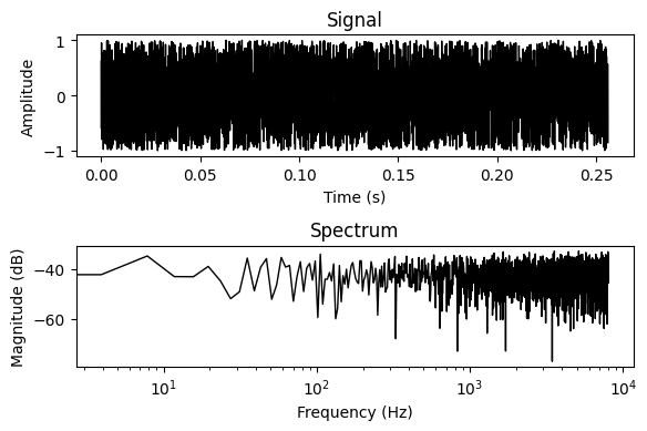
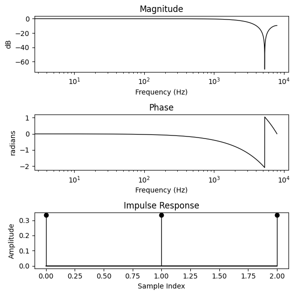
../_images/bea995d65299c719b30662d85741529c9e91aaedab3fe543e83603c0943e3c89.png

Now let’s create a very simple filter, the one given by the difference equation:

\[ y[n] = \frac{1}{3}(x[n] + x[n-1] + x[n-2]). \]

This is a simple moving average filter, which attenuates the high frequencies. It is equivalent to the impulse response: \(\mathbf{h} = \frac{1}{3}\begin{bmatrix}1 & 1 & 1\end{bmatrix}^T\).

Again, we first create a helper function to plot the filter response as a Bode plot.

And then we define our filter…

h = torch.tensor([1.0, 1.0, 1.0]) / 3

bode_plot(h, N)

../_images/0522cc0568ca0ac0f8e90f1483e116e4c8585bafc038576b02f84f07809cfdac.png

We will now use PyTorch’s nn.functional.conv1d to apply our impulse response (aka kernel) to our signal. Note that this function expects an input tensor with the shape [batch, in_channels, time], and a kernel tensor with shape [out_channels, in_channels, length]. Now, as we are operating with a batch size of 1, and on only a single channel, we will just add placeholder dimensions.

x_ = x[None, None, :]  # unsqueeze to [batch, in_channels, time]
h_ = h[None, None, :]  # unsqueeze to [out_channels, in_channels, length]

print(f"input shape: {x_.shape}\nkernel shape: {h_.shape}")

input shape: torch.Size([1, 1, 4096])
kernel shape: torch.Size([1, 1, 3])

Our tensors are correctly shaped… let’s perform the convolution! Note that we call torch.Tensor.flip() in order to reverse the impulse response. This makes the nn.functional.conv1d’s cross-corelation operation into a convolution.

We also pad the signal causally, rather than relying on PyTorch’s same padding, which is non-causal. In non-causal padding, extra samples are added to both the start and end of a signal, which means that the output at any given index depends on past, present, and future indices. In causal padding, \(L-1\) extra samples are added to the start, which means that any given output sample depends only on past and present input samples.

x_padded = nn.functional.pad(x_, (h_.shape[-1] - 1, 0))
y_ = nn.functional.conv1d(
    x_padded,
    h_.flip(-1),
)
y = y_.squeeze()

plot_signal_and_spectrum(y)

../_images/eba655c4216fe97d9e92ae0eb59c7f9524b96f4671afa3e939b58fc67146ee16.png

Optimising our simple FIR filter#

Now, let’s try to optimise the impulse response of our direct convolution filter so that it matches a target filter’s response. To do so, let’s first wrap our filtering code in a nice tidy function:

@torch.jit.script
def apply_conv1d_fir(input_signal: torch.Tensor, impulse_response: torch.Tensor):
    input_signal = nn.functional.pad(input_signal, (impulse_response.shape[-1] - 1, 0))
    input_signal = input_signal[None, None, :]  # unsqueeze to [batch, in_channels, time]
    impulse_response = impulse_response[None, None, :]  # unsqueeze to [out_channels, in_channels, length]
    output_signal = nn.functional.conv1d(
        input_signal,
        impulse_response.flip(-1),
    )
    return output_signal.squeeze()

We then define our predicted filter’s impulse response as a tensor. Note that we set requires_grad=True. This ensures that PyTorch records operations on this tensor in its computation graph so that we can perform backpropogation to recover its gradient.

N = 512
M = 7
predicted_impulse_response = torch.randn(M, requires_grad=True)

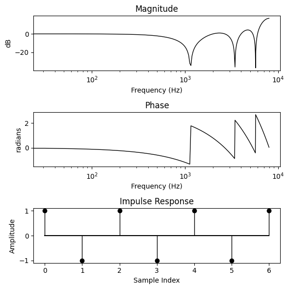
bode_plot(predicted_impulse_response, N)

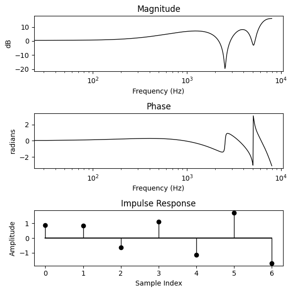
../_images/79f46b285224cf7b639ec5c64d6505b5ef4f93de331b6094becf64522d6edb38.png

We define a synthetic target signal by creating a target filter… Let’s make it something very obvious, alternating 1s and -1s.

target_filter = torch.Tensor([1, -1, 1, -1, 1, -1, 1])
bode_plot(target_filter, N)

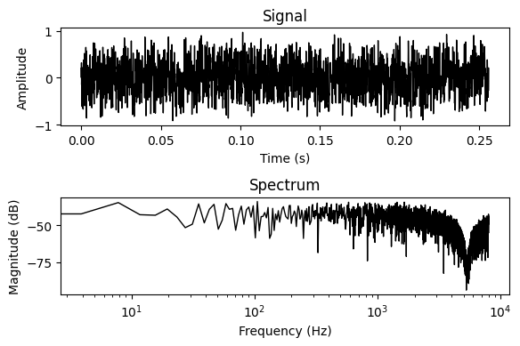
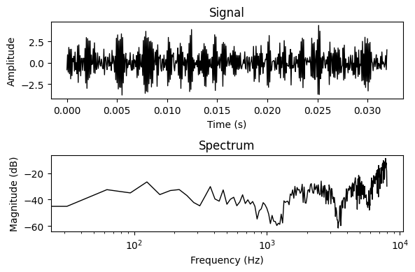
../_images/604c3c95e1848bd5fa4d4a62a7ad6d8a310955e919381de09d60708a3b989d78.png

We define our target signal by applying the filter to some white noise.

input_signal = torch.empty(N).uniform_(-1, 1)
target_signal = apply_conv1d_fir(input_signal, target_filter)

plot_signal_and_spectrum(target_signal)

../_images/af9cb4b66a36ef6b4d87047e6e1991bf588b9a2903f2f47e132313fc62bd631e.png

Now we write a simple optimisation loop. Note that we are applying the filter to the noise signal in order to compute our loss. We are then taking a loss function between our target signal and the noise signal filtered by our predicted filter. This means there’s no reason that we need to use \(L^2\) loss — we can use any loss function we can define on the signal.

optimizer = torch.optim.Adam([predicted_impulse_response], lr=1e-3)
criterion = nn.MSELoss()

steps = 7000
interval = 1000

for step in range(steps):
    predicted_signal = apply_conv1d_fir(input_signal, predicted_impulse_response)
    loss = criterion(target_signal, predicted_signal)

    optimizer.zero_grad()
    loss.backward()

    optimizer.step()

    if step % interval == 0:
        print(f"Step {step}: loss {loss.item():.4f}")

Step 0: loss 9.8862

Step 1000: loss 3.6374

Step 2000: loss 1.0242

Step 3000: loss 0.1884

Step 4000: loss 0.0172

Step 5000: loss 0.0004

Step 6000: loss 0.0000

Cool! That converged quickly. Let’s plot the learnt response…

bode_plot([target_filter, predicted_impulse_response], N, labels=["target", "predicted"])

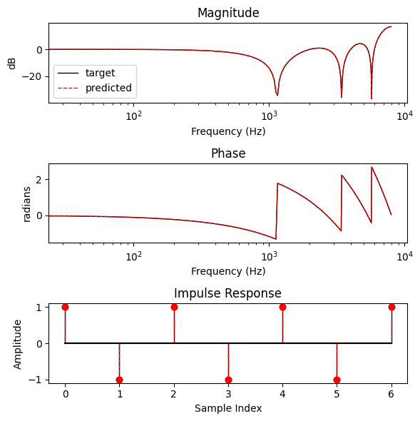
../_images/aff4b5e123cba0e555852105204ad3387ddd72cb66956243b1c21abb3d969f44.png

A perfect fit!

FFT Convolution#

For longer impulse responses, the quadratic time complexity of naive convolution becomes a bottleneck, and so efficient convolution algorithms are often preferred. Perhaps the best known is FFT convolution, which is a result of the discrete convolution theorem — the discrete Fourier transform of the circular convolution of two periodic signals is equal to the element-wise product of the Fourier transforms of the individual signals:

\[ \mathcal{F}\{u\ast v\}[k] = \mathcal{F}\{u\}[k] \cdot \mathcal{F}\{v\}[k] \]

Computationally, this allows us to perform convolution in \(\mathcal{O}(n\log n)\) time in lieu of \(\mathcal{O}(n^2)\). Let’s try implementing it.

@torch.jit.script
def apply_fft_fir(input_signal: torch.Tensor, impulse_response: torch.Tensor):
    N = input_signal.shape[-1]
    L = impulse_response.shape[-1]
    n_fft = N + L - 1
    
    X = torch.fft.rfft(input_signal, n=n_fft)
    H = torch.fft.rfft(impulse_response, n=n_fft)
    y = torch.fft.irfft(X * H)

    return y[:-(L - 1)]

The parameter \(n=...\) of \(torch.fft.rfft\) will zero pad an input signal up to the given length, if it is longer than the input. Here, we zero pad the lengths of the input signal (starting length \(N\)) and the impulse response (starting length \(L\)) to \(N+L-1\). This is because frequency domain multiplication is equivalent to circular convolution. This zero padding is hence necessary to avoid the tail of the convolved signal “wrapping” to the start.

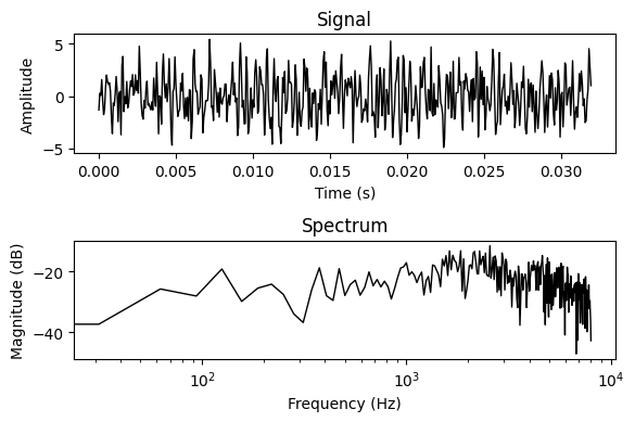
Now let’s apply it to a signal…

h = torch.randn(11)
y = apply_fft_fir(input_signal, h)
plot_signal_and_spectrum(y)

../_images/bda6b6e6287942c45e55df2ab486fd50b10b7f037fe1fecfb125e4c7b61a8862.png

…and compare to our time-domain implementation:

y_ = apply_conv1d_fir(input_signal, h)
plot_signal_and_spectrum(y_)

../_images/b2a046a1db91448e137d8c375beb9559e4700e6c99ac7514e661c6db2854840d.png

Looks close! Let’s check the error…

mse = (y - y_).square().mean().item()
print(f"Mean squared error between nn.functional.conv1d and FFT convolution is: {mse}")

Mean squared error between nn.functional.conv1d and FFT convolution is: 2.2219007775152455e-13

The question is… is it really faster than directly applying the convolution? Let’s run a small experiment to find out…

from timeit import timeit

n_trials = 1000

N = 1024
x = torch.empty(N)

ir_sizes = [2 ** n for n in range(2, 14)]
fft_times = []
conv1d_times = []

for ir_size in ir_sizes:
    h = torch.empty(ir_size)

    fft_time = timeit(lambda: apply_fft_fir(x, h), number=n_trials)
    conv1d_time = timeit(lambda: apply_conv1d_fir(x, h), number=n_trials)

    fft_times.append(fft_time)
    conv1d_times.append(conv1d_time)

    print(f"IR length L = {ir_size}: FFT time {fft_time:.3f}, Conv1D time {conv1d_time:.3f}")

plt.plot(ir_sizes, conv1d_times, color="black", label="Direct")
plt.plot(ir_sizes, fft_times, color="red", label="FFT")
plt.ylabel(f"Time for {n_trials} runs (seconds)")
plt.xlabel("IR Length (samples)")
plt.xscale("log")
plt.legend()

IR length L = 4: FFT time 0.287, Conv1D time 0.031

IR length L = 8: FFT time 0.304, Conv1D time 0.032

IR length L = 16: FFT time 0.304, Conv1D time 0.034

IR length L = 32: FFT time 0.292, Conv1D time 0.038

IR length L = 64: FFT time 0.311, Conv1D time 0.044

IR length L = 128: FFT time 0.305, Conv1D time 0.054

IR length L = 256: FFT time 0.352, Conv1D time 0.076

IR length L = 512: FFT time 0.417, Conv1D time 0.120

IR length L = 1024: FFT time 0.531, Conv1D time 0.251

IR length L = 2048: FFT time 0.814, Conv1D time 0.516

IR length L = 4096: FFT time 1.620, Conv1D time 1.203

IR length L = 8192: FFT time 3.086, Conv1D time 3.569

<matplotlib.legend.Legend at 0x7f00a50b3dc0>

../_images/7ce8e973d32326b033ba6a0b4dcedcd4c5991540903ab866599233a09e293229.png

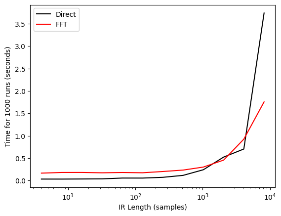
As expected, for larger impulse responses FFT convolution is clearly faster. But interestingly, for responses below roughly 1000 samples, the direct convolution approach wins out.

There are a number of factors at play here, and to detail them all would be well beyond the scope of this tutorial. However, it suffices to acknowledge a few points:

This is a single implementation being tested under unscientific conditions on a particular CPU.
Convolutions are conditionally dispatched to different MKLDNN (CPU) and cuDNN (GPU) kernels depending on various factors including kernel size. These include other fast-convolution algorithms such as Winograd.
We can expect a bigger relative speed up for FFT convolutions on a GPU thanks to hardware-level parallelisation of matrix multiplications. Chin-Yun Yu provides a very illustrative notebook performing these comparisons on a GPU, which suggests that the advantage of FFT convolution becomes apparent around 100 samples.

For more background, and a performance comparison of cuDNN convolution algorithms, see the work of Jordà et al. [JVLP19].

Linear Phase Filter Design by Frequency Sampling#

While we can directly optimise the impulse response, we may wish instead to provide a frequency response from which we derive a filter. For example, we may not be concerned with directly specifying the phase response, or we may wish to enforce linear phase. Further, we may simply wish to have a more interpetible intermediate filter representation, allowing for regularisation or weighting of specific frequency bands.

To address these needs, we turn to the classical signal processing toolbox and adopt the frequency sampling method for linear phase FIR filter design. The first differentiable implementation of this method was provided by Engel et al. [EHGR20], who used it in combination with a harmonic sinusoidal model to create a differentiable harmonic-plus-noise synthesiser.

The design process works as follows. The target magnitude response is given as a vector \(\mathbf{H}^\ast\) of samples from the desired frequency response, taken at the frequencies of a discrete Fourier transform.

We take the inverse discrete Fourier transform of the impulse response (denoted below as the Hermitian transpose, \(\cdot^H\), of the period \(N\) discrete Fourier matrix, \(W_N\)). The resulting signal is a zero phase FIR filter, and is hence non-causal.

Due to the periodicity of the DFT, we can shift it to causal form with a circular shift, which we denote below by the matrix \(C\). This shift changes the zero phase response to a linear phase response.

Finally, we apply a window function \(\mathbf{w}\), written below using the elementwise product \(\odot\). This helps suppress spectral leakage, at the expense of a wider main lobe.

\[\begin{split} \begin{array}{rlr} \mathbf{h}^\ast &= \mathbf{W}_N^H \mathbf{H}^\ast & \text{(magnitude response }\mapsto\text{ impulse response)} \\ \mathbf{h}_s &= \mathbf{C} \mathbf{h}^\ast & \text{(circular shift of }\left\lfloor\frac{M}{2}\right\rfloor \text{)} \\ \mathbf{h} &= \mathbf{w} \odot \mathbf{h}_s & \text{(apply window function)} \\ \end{array} \end{split}\]

Let’s create a simple low-pass filter by specifying a target impulse response with the following frequency response:

\[\begin{split} H^\ast(\omega) = \begin{cases} 1 & |\omega| < \omega_c \\ 0 & \text{otherwise} \end{cases} = \text{rect}\left(\frac{\omega}{\omega_c}\right) \end{split}\]

where \(\omega_c\) is the cutoff frequency. Here we’ll set it to \(2\pi\frac{10}{L}\).

From the definition of this low-pass filter, we would expect to see a normalised sinc function — \(\text{sinc}(x) = \frac{\sin\pi x}{\pi x}\) — as the impulse response. This follows from the inverse discrete-time Fourier transform of the frequency response:

\[ h^\ast[n] = \int_{-\pi}^\pi H^\ast(\omega) e^{j\omega n} d\omega = \int_{-\omega_c}^{\omega_c} e^{j\omega n} d\omega = \frac{\omega_c}{\pi} \text{sinc}(\omega_c n) \]

ir_length = 65

H_target = torch.cat((
    torch.ones(10),
    torch.zeros(ir_length // 2 + 1 - 10),
))
h_zero_phase = torch.fft.irfft(H_target, n=ir_length)
h_s = torch.roll(h_zero_phase, ir_length // 2)
window = torch.hann_window(ir_length)
h = window * h_s
bode_plot(h, 4096)

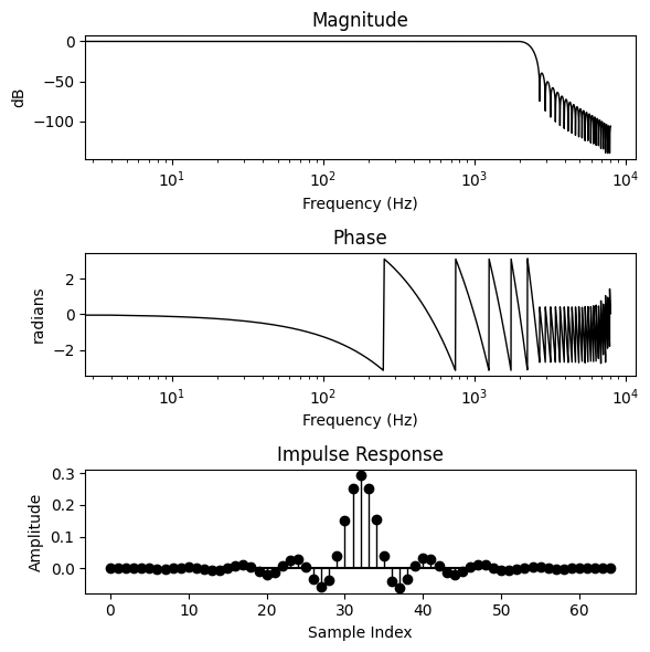
../_images/dae9791ea8aed091db665be2b35773445df60c7d55f9d750535edfb8d84dbf5e.png

Great! We have designed a linear phase filter which approximates our desired magnitude response. Note that while our impulse response has length \(L=65\), the actual length of the array H_target is \(\lfloor L / 2\rfloor + 1\), not \(L\). This is because our desired impulse response is real valued, and so its spectrum is conjugate-symmetric around the Nyquist. We can thus use the more efficient torch.fft.irfft (see docs), which expects a half-Hermitian signal of length \(N / 2 + 1\) and returns a signal of length \(2(N-1)\). Odd-length outputs can be handled by again using the built-in zero padding via the n=... parameter.

Let’s try to learn a magnitude response using this differentiable design procedure. This time we’ll define a slightly more challenging task: given a signal containing a mixture of sinusoidal components, extract a single frequency component.

First, we’ll wrap our differentiable design procedure in a function.

def fir_window_design(
    target_magnitude_response: torch.Tensor,
    window_fn: Callable = torch.hann_window,
) -> torch.Tensor:
    ir_length = (target_magnitude_response.shape[-1] - 1) * 2
    
    h_zero_phase = torch.fft.irfft(target_magnitude_response)
    h_causal = torch.roll(h_zero_phase, ir_length // 2)
    window = window_fn(ir_length)
    h = window * h_causal
    return h

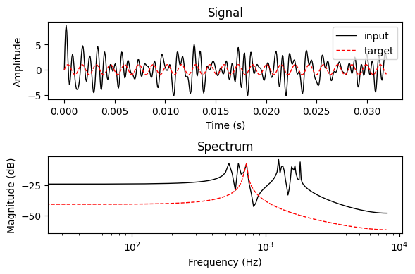
Next, we’ll define our task by specifying the input and target signals.

N = 512
num_components = 10
freqs = torch.empty(num_components).uniform_(0, 1.0)
n = torch.arange(N)
components = torch.sin(freqs[:, None] * n[None])

input_signal = components.sum(dim=0)
target_signal = components[0]

plot_signal_and_spectrum([input_signal, target_signal], labels=["input", "target"])

../_images/b083c80851a5a840589039be8e5d425922c19282203b9d3b5f3a34d22e836a90.png

Then, we’ll define a frequency domain loss function which takes distances only between magnitude spectra.

def fft_loss(a: torch.Tensor, b: torch.Tensor):
    A = safe_abs(torch.fft.rfft(a))
    B = safe_abs(torch.fft.rfft(b))

    return nn.functional.l1_loss(A, B)

Finally, we will initialise our filter…

ir_length = 64
predicted_filter_response = torch.randn(ir_length // 2 + 1, requires_grad=True)

And we are ready to optimise!

optimizer = torch.optim.Adam([predicted_filter_response], lr=1e-3)
criterion = fft_loss

steps = 20000
interval = 1000

for step in range(steps):
    predicted_ir = fir_window_design(predicted_filter_response)
    predicted_signal = apply_conv1d_fir(input_signal, predicted_ir)
    
    loss = criterion(target_signal, predicted_signal)

    optimizer.zero_grad()
    loss.backward()

    optimizer.step()

    if step % interval == 0:
        print(f"Step {step}: loss {loss.item():.4f}")

Step 0: loss 7.3183

Step 1000: loss 2.1302

Step 2000: loss 1.4335

Step 3000: loss 1.3707

Step 4000: loss 1.3236

Step 5000: loss 1.3022

Step 6000: loss 1.2826

Step 7000: loss 1.2639

Step 8000: loss 1.2484

Step 9000: loss 1.2349

Step 10000: loss 1.2247

Step 11000: loss 1.2133

Step 12000: loss 1.2016

Step 13000: loss 1.1901

Step 14000: loss 1.1796

Step 15000: loss 1.1698

Step 16000: loss 1.1622

Step 17000: loss 1.1550

Step 18000: loss 1.1479

Step 19000: loss 1.1423

We seem to be converging on something… Let’s check it out — first we plot the predicted signal against the target signal.

plot_signal_and_spectrum([target_signal, predicted_signal], labels=["predicted", "target"])

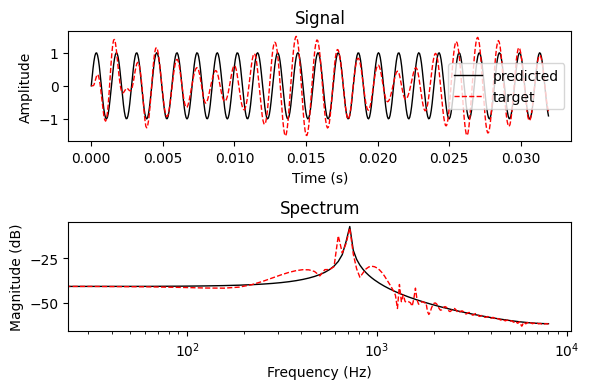
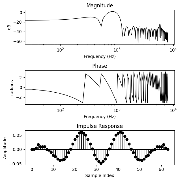
../_images/939364a6d2b71d77d31b877da0dd908f27f302b7a2036292b2f7df411a8bde7d.png

Not bad! We appear to be getting close to extracting the target frequency component. Now let’s look at the filter we have learnt.

bode_plot(predicted_ir, N)

../_images/51e5a0d663f3577669b14e23d7bb97e2e9bf0b331441b04e18ed16ab220c3d9e.png

Time-Varying FIR Filters#

In the context of synthesis we often wish to produce sounds that change over time, and so we would ideally like to be able to vary the filter response. For example, in Engel et al.’s differentiable harmonic-plus-noise synthesiser [EHGR20], the frequency sampling technique we implemented in the previous section is applied to a time series of frequency responses, which are applied to overlapping segments of incoming white noise signal. These filtered segments are windowed and recombined using overlap-add (OLA) to produce the final signal.

We will re-implement this time-varying filtered noise synthesiser here. We first produce the local filter impulse responses using the function we defined above. We then apply these to the input signal using circular convolution in the frequency domain multiplication.

def time_varying_fir(
    input_signal: torch.Tensor,  # [time]
    target_filter_responses: torch.Tensor,  # [frames, ir_length / 2 + 1]
    n_fft: int,
    hop_length: int,
    filter_window_fn: Callable = torch.hann_window,
    ola_window_fn: Callable = torch.hann_window,
) -> torch.Tensor:
    # design the filters
    filter_irs = fir_window_design(target_filter_responses, filter_window_fn)

    num_frames, ir_length = filter_irs.shape
    signal_length = input_signal.shape[0]

    # compute the STFT of the signal
    signal_spectrum = torch.stft(
        input_signal,
        n_fft=n_fft,
        hop_length=hop_length,
        return_complex=True,
    )

    # zero pad the filters and compute their frequency responses
    pad_amount = n_fft - ir_length
    padded_filters = nn.functional.pad(filter_irs, (0, pad_amount))
    filter_responses = torch.fft.rfft(padded_filters, dim=-1).T

    # apply the filters by circular convolution in the freq. domain
    filtered_frames = filter_responses * signal_spectrum

    # take the ISTFT, overlap-adding the resulting frames
    ola_window = ola_window_fn(n_fft)    
    filtered_signal = torch.istft(
        filtered_frames,
        n_fft=n_fft,
        hop_length=hop_length,
        length=signal_length,
        window=ola_window
    )
    return filtered_signal

To test this implementation, let’s use an audio signal. We’ll load a short snippet of a percussion loop.

length_in_seconds = 1.0
signal_length = int(length_in_seconds * SAMPLE_RATE)

target_signal, sr = torchaudio.load("../audio/perc_loop.wav")

target_signal = target_signal[0]
target_signal = torchaudio.functional.resample(target_signal, sr, SAMPLE_RATE)
target_signal = target_signal[:signal_length]

ipd.Audio(target_signal, rate=SAMPLE_RATE)

Then, we’ll randomly initialise our filterbank and apply it to a white noise signal (warning: likely to be loud and unpleasant)

Note that in time_varying_fir we zero pad the impulse response to match the length of n_fft, allowing us to set these to two different lengths.

n_fft = 128
hop_length = 64
ir_length = 33
n_filters = signal_length // hop_length + 1

predicted_filters = torch.randn(n_filters, ir_length // 2 + 1, requires_grad=True)
input_signal = torch.empty(signal_length).uniform_(-1, 1)

with torch.no_grad():
    predicted_signal = time_varying_fir(input_signal, predicted_filters, n_fft, hop_length)

ipd.Audio(predicted_signal, rate=SAMPLE_RATE)

/home/runner/.local/lib/python3.10/site-packages/torch/functional.py:660: UserWarning: A window was not provided. A rectangular window will be applied,which is known to cause spectral leakage. Other windows such as torch.hann_window or torch.hamming_window can are recommended to reduce spectral leakage.To suppress this warning and use a rectangular window, explicitly set `window=torch.ones(n_fft, device=<device>)`. (Triggered internally at ../aten/src/ATen/native/SpectralOps.cpp:837.)
  return _VF.stft(input, n_fft, hop_length, win_length, window,  # type: ignore[attr-defined]

As our filters are time-varying, we’ll need a time-varying loss. It is common with DDSP to use a multi-resolution STFT loss, but for simplicity’s sake we will use a single STFT scale.

def stft_loss(
    a: torch.Tensor, 
    b: torch.Tensor,
    n_fft: int,
    hop_length: int,
):
    A = torch.stft(a, n_fft=n_fft, hop_length=hop_length, return_complex=True)
    B = torch.stft(b, n_fft=n_fft, hop_length=hop_length, return_complex=True)

    A = safe_abs(A)
    B = safe_abs(B)
    return nn.functional.l1_loss(A, B)

Finally, we optimise the filter responses by gradient descent.

optimizer = torch.optim.Adam([predicted_filters], lr=1e-3)
criterion = partial(stft_loss, n_fft=n_fft, hop_length=hop_length)

steps = 15000
interval = 1000

for step in range(steps):
    predicted_signal = time_varying_fir(input_signal, predicted_filters, n_fft=n_fft, hop_length=hop_length)
    
    loss = criterion(target_signal, predicted_signal)

    optimizer.zero_grad()
    loss.backward()

    optimizer.step()

    if step % interval == 0:
        print(f"Step {step}: loss {loss.item():.4f}")

Step 0: loss 3.7415

Step 1000: loss 0.7070

Step 2000: loss 0.1733

Step 3000: loss 0.1155

Step 4000: loss 0.1067

Step 5000: loss 0.1037

Step 6000: loss 0.1021

Step 7000: loss 0.1012

Step 8000: loss 0.1006

Step 9000: loss 0.1001

Step 10000: loss 0.0996

Step 11000: loss 0.0992

Step 12000: loss 0.0988

Step 13000: loss 0.0985

Step 14000: loss 0.0983

Let’s listen to the audio this produces…

print("Predicted")
ipd.display(ipd.Audio(predicted_signal.detach(), rate=SAMPLE_RATE))
print("Target")
ipd.display(ipd.Audio(target_signal.detach(), rate=SAMPLE_RATE))

Predicted

Target

Not bad at all!

Conclusion#

This was a whirlwind tour of differentiable implementations of finite impulse response filters. Differentiable FIR filters have been used for applications from monophonic instrument modelling [EHGR20], through maximum voice frequency estimation [WY19]. For further information and a more thorough review, we refer readers to a recent review article on differentiable digital signal processing [HSF+23].