Writing an Oscillator in PyTorch#
The core of sinusoidal modelling synthesis is the sinusoidal oscillator:
where \(\alpha[n]\) and \(\phi[n]\) are time-varying amplitude and instaneous phase at the \(n^\text{th}\) sample, respectively.
However, we typically want to control an oscillation in terms of frequency instead of specifying the instaneous phase directly.
Recall the relationship between frequency and phase:
Frequency is the derivative of phase. Therefore, phase can be calculated by integrating the instaneous frequency and adding an intial phase offset:
where \(\omega[n]\) is the instantaneous angular frequency at the \(n^\text{th}\) sample and \(\phi_0\) is the initial phase.
Our final equation for our sinusoidal oscillator is:
Different types of frequency#
You might have noticed that we specified frequency, \(\omega\), as angular frequency. Angular frequency is measured in radians per second or radians per sample.
When we’re dealing with audio we’ll also deal with frequency specified in Hertz (Hz), which is cycles per second. For example, you might know that in the Western music tradition the A above middle C is tuned to 440Hz (or maybe 432Hz is more your thing).
How are frequency in Hertz and angular frequency related?
Digital audio is sampled at a particular sampling rate. For example, we’re dealing with audio sampled at 16kHz in this notebook. The Nyquist theorem states that we can accurately represent audio frequencies up to half the sampling frequency. So if \(f_s = 16000\text{Hz}\), we can accurately represent frequencies up to \({f_s}/{2} = 8000\text{Hz}\).
To determine angular frequency from a frequency in Hz we need to know the sampling rate of the system and normalize such that \(2\pi = f_s\). This means that the range of angular frequencies that can be accurately represented fall in the range \([0,\pi)\). Frequencies that are outside that range cause aliasing (incorrect representation of those frequencies).
For example 440Hz at 16kHz sampling rate in angular frequency:
import math

omega = 2 * math.pi * (440.0 / 16000.0)
print(f"omega = {omega} rad/sample")
omega = 0.17278759594743862 rad/sample
For a nice visual introduction and overview of some of these core DSP concepts we recommend Jack Schaedler’s fantastic primer on the topic: Seeing Circles, Sines, and Signals.
Sample Rate vs. Frame Rate#
In the above equation for our sinusoidal oscillator we have time-varying amplitude and frequency values at the same resolution as the audio sampling rate.
In practice, we specify amplitude and frequency values at a significantly lower rate – referred to as the frame rate – and then upsample these envelopes to match the sampling rate before synthesis.
For example, we might use a frame rate of 100Hz. This sets an upper bound on the rate of change of our control envelopes and also reduces the dimensionality of our parameter space. With a 100Hz frame rate we only need to estimate 100 values per second as opposed to 16k! (assuming a sampling rate of 16kHz).
There are several different methods for upsampling from frame rate to sampling rate. We’ll use a simple linear interpolation here. Engel et al. used a method with overlapping Hann windows, which they said worked particularly well for amplitude envelopes.
Creating a Sinusoidal Oscillator#
Let’s write the above oscillator function using the PyTorch API.
We’ll then look at how we can parameterize this oscillator and learn to match the amplitude envelope of a target audio sample using gradient descent. Instead of using a global amplitude parameter like we did in the previous chapter, we’ll look at how we can learn a time-varying amplitude envelope.
A note on batching
One of the benefits of using PyTorch is that it provides built-in support for hardware acceleration such as GPUs which enable parallelization of computation. In practice, to utilize this, we need to write our algorithms so that they support batches. Even though we’re not using GPUs and our batch size is one in these notebooks, we include a batch dimension to show what this looks like.
Show code cell source
import torch
import IPython.display as ipd
import matplotlib.pyplot as plt
from matplotlib.animation import FuncAnimation
def sinusoid(
    amplitude: torch.Tensor,  # Amplitude (batch_size, n_frames)
    frequency: torch.Tensor,  # Angular frequency (batch_size, n_frames)
    n_samples: int,  # Number of samples to generate (will upsample to this)
    phase: torch.Tensor = None,  # Initial phase (batch_size,), if None then 0
) -> torch.Tensor:
    """
    Implementational of a sinusoidal oscillator function. Receives time-varying
    amplitude and angular frequency as input and synthesizes a sinusoidal signal.
    An optional initial phase can also be specified.
    """
    # If initial phase is not specified, set it to 0
    if phase is None:
        phase = torch.zeros(amplitude.shape[0])

    # Upsample the amplitude and angular frequency tensors to the desired number of samples
    amplitude = torch.nn.functional.interpolate(
        amplitude.unsqueeze(0), size=n_samples, mode="linear"
    ).squeeze(0)
    frequency = torch.nn.functional.interpolate(
        frequency.unsqueeze(0), size=n_samples, mode="linear"
    ).squeeze(0)

    # Unsqueeze the last dimension of phase to give it a time step dimension equal to 1
    # Then add the initial phase to the beginning of the angular frequency tensor
    # This sets the initial phase of the oscillator
    # We then discard the last element of the angular frequency tensor to maintain
    # the correct number of time steps
    phase = phase.unsqueeze(-1)
    frequency = torch.cat([phase, frequency], dim=1)[..., :-1]

    # Calulate the instantaneous phase by integrating the angular frequency.
    phase = torch.cumsum(frequency, dim=1)
    return amplitude * torch.sin(phase)
Using our oscillator#
To use our new sinusoidal oscillator we need to create the control envelopes for the function, which are tensors representing the time-varying angular frequency and amplitude values.
Let’s first make a static tone at 440Hz at an audio sampling rate of 16kHz.
sample_rate = 16000  # Audio sampling rate
frame_rate = 100  # Frame rate of control signal
f0 = 440.0  # Frequency of the sinusoid in Hz
Make a frequency envelope at 440Hz for one second. Then, convert to angular frequency, which has a range of \([0, 2\pi)\), where \(2\pi\) is the sampling rate.
frequency = torch.ones(1, frame_rate) * f0
frequency = frequency * 2 * torch.pi / sample_rate

print(f"Shape of the frequency envelope: {frequency.shape}")
Shape of the frequency envelope: torch.Size([1, 100])
Similarly, make a static amplitude signal with an amplitude of 0.5
amplitude = torch.ones(1, frame_rate) * 0.5

print(f"Shape of the amplitude envelope: {frequency.shape}")
Shape of the amplitude envelope: torch.Size([1, 100])
Synthesize it!
y = sinusoid(amplitude, frequency, n_samples=sample_rate)
ipd.Audio(y[0].numpy(), rate=sample_rate, normalize=False)
Show code cell source
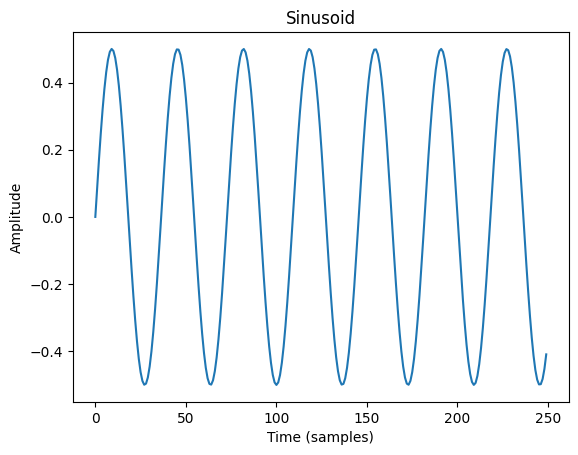
plt.plot(y[0, :250].numpy())
plt.title("Sinusoid")
plt.xlabel("Time (samples)")
plt.ylabel("Amplitude")
plt.show()
Varying the frequency and amplitude#
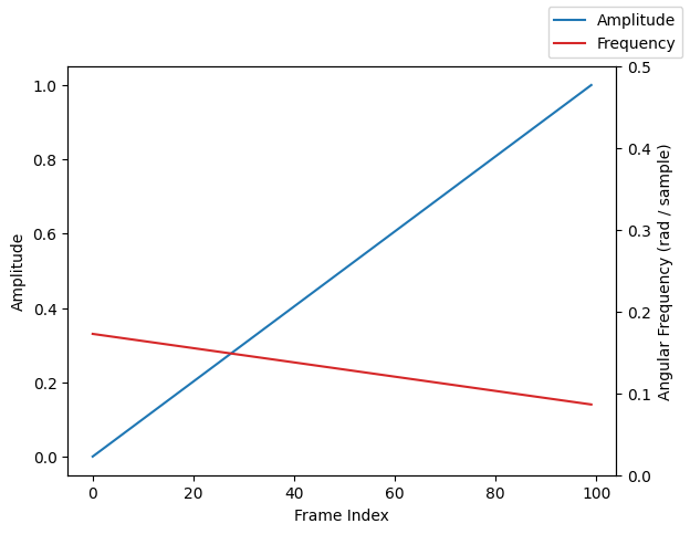
Because our amplitude and frequency tensors represent time-varying values, we can synthesize a sound with modulating amplitude and frequency. For example, let’s have the frequency decrease by an octave from 440Hz to 220Hz over one second while the amplitude increases from zero.
# Frequency envelope - Hz
frequency = torch.linspace(440, 220, frame_rate).unsqueeze(0)

# Convert to angular frequency - rads / sample
frequency = frequency * 2 * torch.pi / sample_rate

# Amplitude envelope
amplitude = torch.linspace(0, 1, frame_rate).unsqueeze(0)
Show code cell source
# Plot the amplitude and angular frequency envelopes
fig, ax1 = plt.subplots()

ax1.plot(amplitude[0].numpy(), color="tab:blue", label="Amplitude")
ax1.set_ylabel("Amplitude")
ax1.set_xlabel("Frame Index")

ax2 = ax1.twinx()
ax2.plot(frequency[0].numpy(), color="tab:red", label="Frequency")
ax2.set_ylabel("Angular Frequency (rad / sample)")
ax2.set_ylim(0, 0.5)

fig.legend()
plt.show()
y = sinusoid(amplitude, frequency, n_samples=sample_rate)
ipd.Audio(y[0].numpy(), rate=sample_rate, normalize=False)
Optimizing parameters for our oscillator#
Now we have a differentiable sinusoidal oscillator!
Let’s optimize the amplitude envelope to match a target audio.
Our target audio will be audio we just generated with the increasing amplitude and decreasing frequency.
y = sinusoid(amplitude, frequency, n_samples=sample_rate)
Loss Functions#
For our loss function we’ll use an \(L_1\) loss computed on the time domain audio signal. Recall that this loss is sensitive to phase variances; however, we know that phase will be identical between these signals because we’re using the same frequency envelope with zero initial phase.
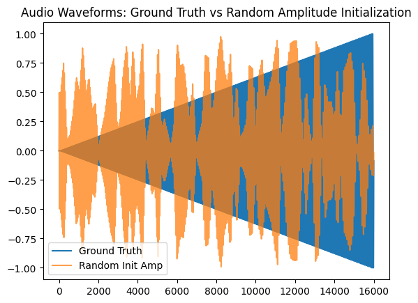
Amplitude Initialization#
We’ll create a random amplitude envelope that will serve as the parameter initialization prior to optimization.
# Create a random amplitude envelope with 8 random points and interpolate it to the
# audio sampling rate
torch.random.manual_seed(0)
rand_amp = torch.rand(1, frame_rate)

y_hat = sinusoid(rand_amp, frequency, n_samples=sample_rate)

ipd.Audio(y_hat[0].numpy(), rate=sample_rate, normalize=False)
Show code cell source
plt.plot(y[0].numpy(), label="Ground Truth")
plt.plot(y_hat[0].numpy(), alpha=0.75, label="Random Init Amp")
plt.legend()
plt.title("Audio Waveforms: Ground Truth vs Random Amplitude Initialization")
plt.show()
Create a PyTorch parameter and optimizer#
Here we turn our intialized amplitude envelope into a PyTorch Parameter. This tells PyTorch that we want to optimize these values and that it needs to compute gradients with respect to this tensor. We’ll also define an optimizer in this step and pass our amplitude parameters into the optimizer.
In the introduction to PyTorch chapter, we optimized a single gain parameter which was applied equally to all values of the input audio signal. Now we have a time-varying gain envelope which modifies how the gain changes over time, enabling the creation of more complex sounds.
amp_param = torch.nn.Parameter(rand_amp)
optimizer = torch.optim.Adam([amp_param], lr=0.01)
The optimization loop#
loss_log = []
audio_log = []
for i in range(200):
    # Forward pass
    y_hat = sinusoid(amp_param, frequency, n_samples=sample_rate)

    # Compute the loss
    loss = torch.nn.functional.l1_loss(y_hat, y)
    loss_log.append(loss.item())

    # Backward pass and optimization step
    optimizer.zero_grad()
    loss.backward()
    optimizer.step()

    # Save the audio
    if i % 10 == 0:
        audio_log.append(y_hat[0].detach().numpy())
Show code cell source
fig, axes = plt.subplots(1, 2, figsize=(10, 4))

axes[0].plot(y[0].numpy(), label="Ground Truth")

axes[1].set_ylim(0.0, max(loss_log))
axes[1].set_xlim(0, len(loss_log))

(line0,) = axes[0].plot([], [], lw=2, alpha=0.75)
(line1,) = axes[1].plot([], [], lw=2)


def animate(i):
    iteration = i * 10

    axes[0].set_title("Iteration: {}".format(iteration))
    line0.set_data(torch.arange(sample_rate), audio_log[i])

    axes[1].set_title("Loss: {:.4f}".format(loss_log[iteration]))
    line1.set_data(torch.arange(iteration), loss_log[:iteration])

    return (
        line0,
        line1,
    )


# Create the animation
anim = FuncAnimation(fig, animate, frames=len(audio_log), interval=250, blit=True)

plt.close(fig)
# To display the animation in the Jupyter notebook:
display(ipd.HTML(anim.to_html5_video()))
Results#
Synthesize the result with the optimized amplitude parameter. It worked well!
y_hat = sinusoid(amp_param, frequency, n_samples=sample_rate)

# Now that the tensor is a learnable parameter, it is marked as requiring a gradient.
# We need to detach it from the computation graph before plotting and rendering audio.
ipd.Audio(y_hat[0].detach().numpy(), rate=sample_rate, normalize=True)
Optimizing Frequency#
Great! We made a differentiable oscillator and we can use gradient descent to learn an amplitude envelope to match a target.
Now how about optimizing a frequency envelope?
Unfortunately, we have encountered one of the fundamental open challenges in DDSP: optimizing frequency.
Due to the nature of sinusoidal functions, the gradient of our loss with respect to frequency parameters is periodic, which means that the error landscape is full of nasty local minima.
We can plot the \(L_1\) spectral and waveform loss at various frequency values to visualize this.
def static_sin(frequency: float, n_samples: int, sample_rate: int):
    phase = torch.arange(n_samples).float() * frequency / sample_rate
    return torch.sin(phase * 2 * torch.pi)
def spectral_loss(x, y):
    x_fft = torch.fft.rfft(x).abs()
    y_fft = torch.fft.rfft(y).abs()
    return torch.nn.functional.l1_loss(x_fft, y_fft)
# Create a ground truth sinusoid with a frequency of 100 Hz
y = static_sin(100, 1000, sample_rate)

# Create a list of frequencies to test
freqs = list(range(20, 400))

s_loss = []
w_loss = []
for f in freqs:
    y_hat = static_sin(f, 1000, sample_rate)
    s_loss.append(spectral_loss(y_hat, y))
    w_loss.append(torch.nn.functional.l1_loss(y_hat, y))

fig, axes = plt.subplots(1, 2, figsize=(10, 4))
axes[0].plot(freqs, s_loss)
axes[0].set_xlabel("Frequency (Hz)")
axes[0].set_ylabel("Loss")
axes[0].set_title("Spectral Loss")

axes[1].plot(freqs, w_loss)
axes[1].set_xlabel("Frequency (Hz)")
axes[1].set_title("Waveform Loss")

plt.tight_layout()
plt.show()
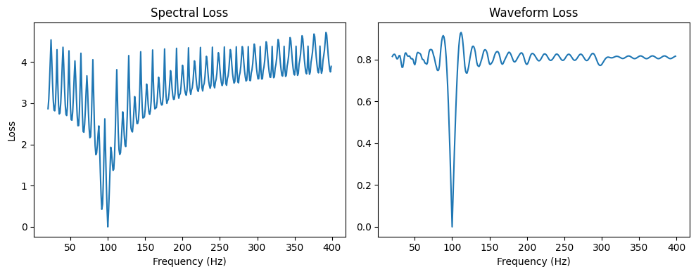
These plots clearly show the correct value of 100Hz as a the global minimum. But the loss surface is littered with local minima, which make gradient descent challenging.
While research is investigating solutions to this problem, diving into this problem is beyond the scope of this part of tutorial.
Despite this problem, lot’s of interesting work has been conducted in DDSP that doesn’t rely on directly learning frequencies of oscillators. In the next section we’ll see how this simple sinusoidal oscillator will form the basis of a more complex synthesizer that can generate realistic instrumental sounds.
Cummulative Summation and Numeric Errors#
In these examples we are using torch’s built-in cumsum function to calculate instantaneous
phase by integrating angular frequency. It is important to note that for longer audio clips
(~ >100k samples) this can lead to an accumulation of phase errors that can become audible
during these longer clips.
Engel et al. introduced an angular_cumsum method to deal with these accumulation errors.
This works by first chopping up an input frequency signal into blocks before computing
instaneous phase via integration, and then stitches the results together, taking into
account the required offsets between blocks to ensure a continuous phase signal.
For more information and code, check out their implementation.
Summary#
In this section we looked at implementing a sinusoidal oscillator in PyTorch that was capable of synthesizing a signal with time-varying amplitude and frequency. We looked at how we can use gradient descent to learn to match an amplitude envelope. In contrast to amplitude, optimizing frequency of a differentiable oscillator is a challenging problem due to the presence of local minima.