Optimizing a Harmonic Synthesizer

Optimizing a Harmonic Synthesizer#

In this section we look at using gradient descent to learn parameters for a harmonic synthesizer to match an instrumental sound.

We’ll define a harmonic synthesizer which has the following additions, which are taken directly from Engel et al. [EHGR20]:

constraining harmonic amplitudes to sum to one;
adding a global amplitude parameter;
parameter scaling to constrain the possible range of amplitudes;
removing frequencies above the Nyquist frequency which will result in aliasing;

The updated formula for our harmonic synthesizer is:

\[ y[n] = A[n]\sum_{k=1}^{K}\hat{\alpha}_k[n]\sin\left(k\sum_{m=0}^{n}\omega_{0}[m]\right) \]

where \(A[n]\) is a global amplitude parameter, and \(\hat{\alpha}_k[n]\) is the normalized amplitude for the \(k^{\text{th}}\) sinusoidal component. \(\hat{\alpha}_k[n]\) is normalized such that \(\sum_{k}\hat{\alpha}_k[n] = 1\) and \(\hat{\alpha}_k[n] > 0\). Fundamental frequency \(\omega_{0}[n]\) is pre-computed using a pitch extraction algorithm.

Methods for parameter scaling and removing frequencies above the Nyquist frequency will be introduced inline below.

Finally, we’ll use gradient descent with a multiresolution spectral loss function to match sounds from the NSynth test dataset [ERR+17].

Parameter Scaling#

Before writing the harmonic synth we’ll define some helper functions.

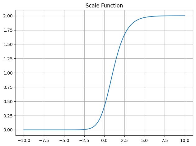
The first is a scaling function that is used to constrain parameter outputs to a particular range while providing stable and informative gradients for a wide range of input values.

def scale_function(
    x: torch.Tensor,
    exponent: float = 10.0,
    max_value: float = 2.0,
    threshold: float = 1e-7,
):
    """
    Scales a parameter to a range of [threshold, max_value] with a slope of exponent.
    A threshold is used to stabilize the gradient near zero.
    """
    return max_value * torch.sigmoid(x) ** math.log(exponent) + threshold

x = torch.linspace(-10.0, 10.0, 100)

plt.plot(x, scale_function(x))
plt.grid()
plt.title("Scale Function")
plt.tight_layout()
plt.show()

../_images/b22f34993f6913bd220ea896a092b4cd3ab0baf681bc02aa82acc90cbb6f60a9.png

Aliasing#

The second function removes any frequencies above the Nyquist frequency, which will be incorrectly represented (i.e, aliased). This zeros out the amplitudes of any frequencies above the Nyquist frequency.

def remove_above_nyquist(
    harmonic_amps: torch.Tensor,
    frequencies: torch.Tensor,
):
    return harmonic_amps * (frequencies < torch.pi).float()

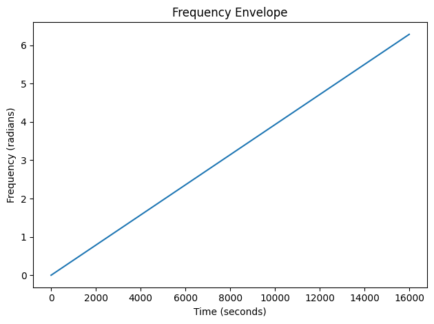
To see what aliasing looks like consider a frequency envelope that goes from 0Hz to the the sample rate \(f_s\) over one second. Remember that the Nyquist frequency is \(f_s / 2\).

freq = torch.linspace(0.0, 2.0 * math.pi, 16000)
amps = torch.ones_like(freq)

../_images/89856d1381b47c537bfecd2b2dbeac921adcb873ae86c09733445f3e3804774a.png

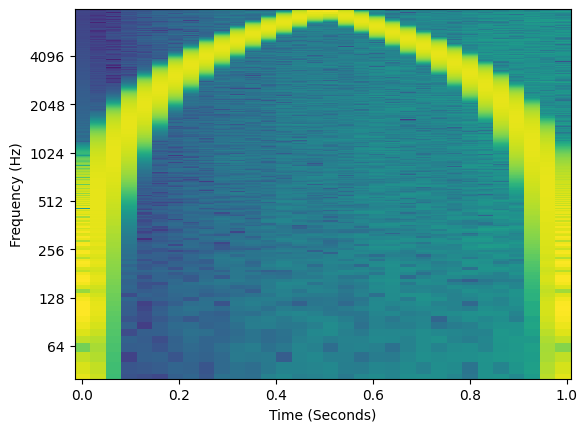
The frequency envelope linearly increases over one second, but when we listen to it and plot the spectrogram we see something different! What happened?? All frequencies above \(\pi\) (Nyquist) have aliased, which we see as wrapping around the Nyquist frequency.

y = amps * torch.sin(torch.cumsum(freq, dim=-1))
plot_spectrogram(y.unsqueeze(0), 16000)
ipd.Audio(y, rate=16000)

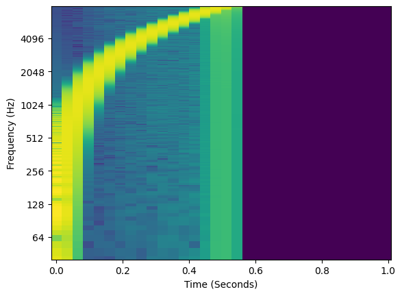
../_images/7206d80901b3d1ed49caa04f5108e4f6c3dd6ef76d142a6843e63b445e4bdbed.png

When we remove frequencies above the Nyquist frequency we get rid of the second half of the signal that was aliasing.

amps = remove_above_nyquist(amps, freq)
y = amps * torch.sin(torch.cumsum(freq, dim=-1))

plot_spectrogram(y.unsqueeze(0), 16000)
ipd.Audio(y, rate=16000)

../_images/f9be453a3c41056d59b5ab752d6c57fd35e36a99606d7f1bbe7a3bdc833fcf85.png

Updated Harmonic Synthesizer#

This function should be familiar from the previous section. Here we calculate \(K\) (n_harmonics) frequencies in relation to a fundamental frequency.

def get_harmonic_frequencies(f0: torch.Tensor, n_harmonics: int):
    # Create integer harmonic ratios and reshape to (1, n_harmonics, 1) so we can
    # multiply with fundamental frequency tensor repeated for n_harmonics
    harmonic_ratios = torch.arange(1, n_harmonics + 1).view(1, -1, 1)

    # Duplicate the fundamental frequency for each harmonic
    frequency = f0.unsqueeze(1).repeat(1, n_harmonics, 1)

    # Multiply the fundamental frequency by the harmonic ratios
    frequency = frequency * harmonic_ratios

    return frequency

def additive_synth(
    amplitudes: torch.Tensor,  # Amplitudes (batch, n_sinusoids, n_frames)
    frequencies: torch.Tensor,  # Angular frequencies (batch, n_sinusoids, n_frames)
    n_samples: int,  # Number of samples to generate (upsample from n_frames)
):
    """
    Generate audio from sinusoidal parameters using additive synthesis.
    """
    # Upsample to n_samples
    amplitudes = torch.nn.functional.interpolate(
        amplitudes, size=n_samples, mode="linear"
    )
    frequencies = torch.nn.functional.interpolate(
        frequencies, size=n_samples, mode="linear"
    )

    # Set initial phase to zero, prepend to frequency envelope
    initial_phase = torch.zeros_like(frequencies[:, :, :1])
    frequencies = torch.cat([initial_phase, frequencies], dim=-1)

    # Create the phase track and remove the last sample (since we added initial phase)
    phase = torch.cumsum(frequencies, dim=-1)[..., :-1]
    y = torch.sin(phase) * amplitudes
    y = torch.sum(y, dim=1)
    return y

Our harmonic_synth has been updated to accept a global_amp parameter (i.e, \(A[n]\)) and the expected number of samples at the output, which is used to upsample from frame rate to sample rate.

We also apply the scaling function to both amplitude parameters, remove frequencies above the Nyquist frequency, and normalize harmonic amplitudes to a distribution.

def harmonic_synth(
    f0: torch.Tensor,  # Angular fundamental frequency (batch, n_samples)
    global_amp: torch.Tensor,  # Global amplitude (batch, n_samples)
    harmonic_amps: torch.Tensor,  # Amplitudes of harmonics (batch, n_harmonics, n_samples)
    n_samples: int,  # Number of samples to synthesize
):
    # Get the harmonic frequencies
    frequencies = get_harmonic_frequencies(f0, harmonic_amps.shape[1])

    # Scale the amplitudes
    harmonic_amps = scale_function(harmonic_amps)
    global_amp = scale_function(global_amp)

    # Remove frequencies above Nyquist
    harmonic_amps = remove_above_nyquist(harmonic_amps, frequencies)

    # Normalize the harmonic amplitudes
    harmonic_amps = harmonic_amps / torch.sum(harmonic_amps, dim=1, keepdim=True)

    # Multiply all harmonic amplitudes by the global amplitude
    harmonic_amps = harmonic_amps * global_amp.unsqueeze(1)

    return additive_synth(harmonic_amps, frequencies, n_samples)

Sound Matching with Gradient Descent#

Now we’ve defined our harmonic synthesizer with the added functionality to more closely mimic the one specified by Engel et al. [EHGR20].

Let’s try to replicate this saxophone sound!

# Load audio
audio, sample_rate = torchaudio.load("../_static/audio/reed_acoustic_011-045-050.wav")

# Extract the first 2.0 seconds of the audio
audio = audio[:1, : int(sample_rate * 2.0)]
ipd.Audio(audio.numpy(), rate=sample_rate)

We first need to determine the fundamental frequency envelope. Engel et al. used crepe [KSLB18], which is a deep learning model trained for pitch extraction.

For this example, we’ll just use torchaudio’s built-in pitch detection to keep things simple. In the next section we’ll share some results using crepe.

# Set parameters to have a frame rate of 100 Hz
f0 = torchaudio.functional.detect_pitch_frequency(
    audio, sample_rate, frame_time=0.0093, win_length=30
)

frame_rate = f0.shape[-1] / (audio.shape[-1] / sample_rate)
print(f"Frame rate: {frame_rate:.2f} Hz")

Frame rate: 100.00 Hz

plt.plot(f0[0, :].numpy())
plt.title("Estimated Fundamental Frequency")
plt.xlabel("Time (frame index)")
plt.ylabel("Frequency (Hz)")
plt.tight_layout()
plt.show()

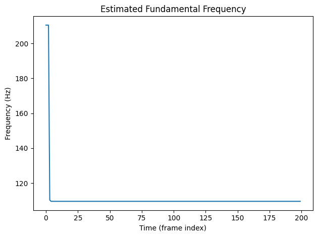
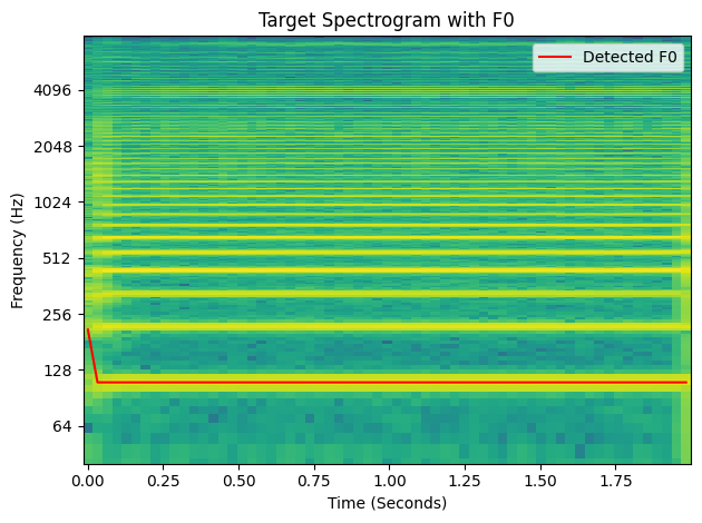
../_images/046af7e884de02d8364201a55671fe16fb4740dec830eb46a8198e6156e13c33.png

We can see in the fundamental frequency plot the pitch detection algorithm has estimated an extremely high value for pitch during the onset. This is an error and will be reflected in the synthesized results. But for demonstration purposes this will work just fine!

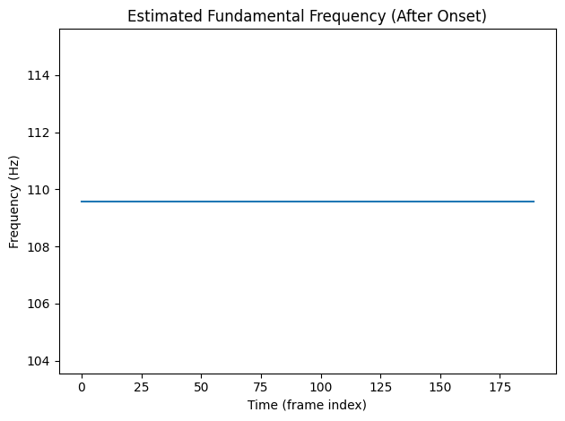
If we look at the fundamental frequency envelope after the onset there is a stable fundamental frequency of about ~110Hz, which corresponds to a pitch of A2.

print(f"Mean fundamental frequency: {f0[0,10:].mean():.2f} Hz")

plt.plot(f0[0, 10:].numpy())
plt.title("Estimated Fundamental Frequency (After Onset)")
plt.xlabel("Time (frame index)")
plt.ylabel("Frequency (Hz)")
plt.tight_layout()
plt.show()

Mean fundamental frequency: 109.59 Hz

../_images/4bc0575706aaabaa8223ddbfdbd077396afa77c4a8b4029d7fe2ca38c57ee2bc.png

Fundamental frequency with the spectrogram#

../_images/132a9318f8176605ac7301f14a3007c53b7f715d3fd32ac5a8a8878bd1850804.png

Spectral Loss#

Before we start optimization we need to define our loss function. A phase variant loss like \(L_1\) on the waveform won’t work here as we’re not expecting our synthesizer to be able to match phase. Besides, we’re focusing on matching sinusoidal components, which is much better handled in the frequency domain.

Recall the spectral loss function we used in the previous chapter which computed the \(L_1\) loss on magnitude spectrums. This provided a phase-invariant audio loss.

Here, we extend this spectral loss to use the short-time Fourier transform, which computes the FFT on small chunks of audio input and allows for time-varying frequency changes to be captured.

Engel et al. used a combination of log magnitude and linear magnitude spectral loss, these are defined as follows:

Log magnitude spectral loss#

\[ \mathcal{L}_\text{log}(\mathbf{y}, \hat{\mathbf{y}}) = \left\lVert \log\left| STFT(\mathbf{y}) \right| - \log\left| STFT(\hat{\mathbf{y}}) \right| \right\rVert_{1} \]

Linear magnitude spectral loss#

\[ \mathcal{L}_\text{lin}(\mathbf{y}, \hat{\mathbf{y}}) = \left\lVert \left| STFT(\mathbf{y}) \right| - \left| STFT(\hat{\mathbf{y}}) \right| \right\rVert_{1} \]

where \(\left\lVert \cdot \right\rVert_1\) denotes the \(L_1\) norm and \(\left|STFT(\cdot)\right|\) is the magnitude spectrogram from the short-time Fourier transform. Spectral convergence [ArikJD18] is another spectral loss that is commonly used but not included in here.

Multiresolution Spectral Loss#

Wang et al. [WTY19] proposed computing a spectral loss using multiple STFT window sizes and hop lengths, aggregating the outputs into a single loss value. This technique has since come to be known as the multi-resolution STFT (MRSTFT) or multi-scale spectral loss (MSS) loss. The motivation behind this formulation is to compensate for the time-frequency resolution tradeoff inherent to the STFT.

A general form for MRSTFT losses is a weighted sum of the different spectral loss formulations at different resolutions:

\[ \mathcal{L}_\text{MRSTFT} = \sum_{k\in{K}}{\alpha_\text{log}\mathcal{L}_{\text{log},k} + \alpha_\text{lin}\mathcal{L}_{\text{lin},k}} \]

where \(K\) is the set of STFT configurations, \(\mathcal{L}_{\cdot,k}\) is a spectral loss computed with a particular configuration, and \(\alpha\) is the weighting for a loss term.

Engel et al. used a selection of FFT sizes ranging from 64 to 2048 samples with 75% overlap. Let’s see what this looks like using the auraloss package

n_ffts = [2048, 1024, 512, 256, 128, 64]
hop_sizes = [n // 4 for n in n_ffts]
loss_fn = auraloss.freq.MultiResolutionSTFTLoss(
    fft_sizes=n_ffts,
    hop_sizes=hop_sizes,
    win_lengths=n_ffts,
    w_sc=0.0,
    w_lin_mag=1.0,
    w_log_mag=1.0,
)

Optimization#

Now we just need to setup the parameters for optimization - global amplitude \(A[n]\) and the harmonic amplitudes \(\alpha_k[n]\). For this example we’ll set \(K=80\).

# Convert fundamental frequency to angular frequency
w0 = f0 * 2 * torch.pi / sample_rate

# Create a harmonic amplitude envelope
n_harmonics = 80
harmonic_amplitudes = torch.randn(1, n_harmonics, f0.shape[-1])

# Create PyTorch parameters - these are the variables we will optimize
harmonic_amplitudes = torch.nn.Parameter(harmonic_amplitudes)
global_amp = torch.nn.Parameter(torch.randn_like(w0))

optimizer = torch.optim.Adam([harmonic_amplitudes, global_amp], lr=0.05)

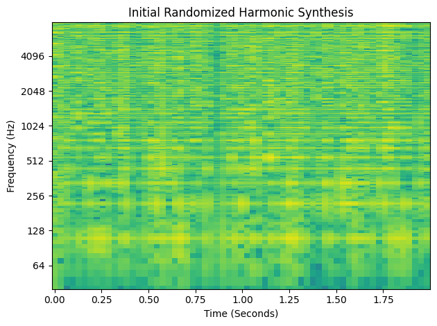
y_hat = harmonic_synth(w0, global_amp, harmonic_amplitudes, audio.shape[-1])
fig, ax, *_ = plot_spectrogram(y_hat.detach(), sample_rate)

ax.set_title("Initial Randomized Harmonic Synthesis")
plt.tight_layout()
plt.show()

../_images/be733ab55b283376ff59b8072d1d267157493c129f1eeac53450eb24d4f39a77.png

Run the optimization loop!

loss_log = []
audio_log = []
for i in range(1000):
    # Forward pass
    y_pred = harmonic_synth(w0, global_amp, harmonic_amplitudes, audio.shape[-1])

    # Compute loss
    loss = loss_fn(audio.unsqueeze(0), y_pred.unsqueeze(0))
    loss_log.append(loss.item())

    # Backward pass and optimization step
    optimizer.zero_grad()
    loss.backward()
    optimizer.step()

    # Log audio and loss
    if i % 50 == 0:
        audio_log.append(y_pred.detach().cpu().numpy())

print("Resulting Harmonic Synthesis:")
ipd.display(ipd.Audio(y_pred[0].detach().numpy(), rate=sample_rate))

print("Target Audio:")
ipd.display(ipd.Audio(audio[0].detach().numpy(), rate=sample_rate))

Resulting Harmonic Synthesis:

Target Audio:

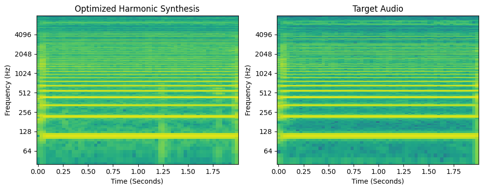
You can hear the outlier pitch at the onset as a squelch, but the steady part of the signal has been matched pretty well!

../_images/1d62bf4b7db79d1e6c53f980926551b25edc786fc950518ae8c2fec3803a3d8c.png

Summary#

We’ve successfully written a differentiable harmonic synthesizer in PyTorch that is capable of learning to match an acoustic instumental sound! In this notebook we introduced a number of additions to the basic harmonic synth based on Engel et al.’s differentiable harmonic synthesizer which helped us in this process. A mutli-resolution STFT loss was then used to optimize the amplitude parameters to match those of a target sound.

In the next section will see how using a better pitch detection algorithm can help and see some more results.

References#

ArikJD18: Sercan Ö Arık, Heewoo Jun, and Gregory Diamos. Fast spectrogram inversion using multi-head convolutional neural networks. IEEE Signal Processing Letters, 26(1):94–98, 2018.
EHGR20(1,2): Jesse Engel, Lamtharn (Hanoi) Hantrakul, Chenjie Gu, and Adam Roberts. DDSP: Differentiable Digital Signal Processing. In 8th International Conference on Learning Representations. April 2020.
ERR+17: Jesse Engel, Cinjon Resnick, Adam Roberts, Sander Dieleman, Mohammad Norouzi, Douglas Eck, and Karen Simonyan. Neural audio synthesis of musical notes with wavenet autoencoders. In International Conference on Machine Learning, 1068–1077. PMLR, 2017.
KSLB18: Jong Wook Kim, Justin Salamon, Peter Li, and Juan Pablo Bello. Crepe: a convolutional representation for pitch estimation. In 2018 IEEE International Conference on Acoustics, Speech and Signal Processing (ICASSP), 161–165. IEEE, 2018.
WTY19: Xin Wang, Shinji Takaki, and Junichi Yamagishi. Neural source-filter waveform models for statistical parametric speech synthesis. IEEE/ACM Transactions on Audio, Speech, and Language Processing, 28:402–415, 2019.