The Wave Equation

In the previous notebook, we explored the dynamics of a system of interconnected undamped oscillators in 1D. Each of these oscillators was connected to its neighbors by springs. When considering an individual simple harmonic oscillator, the restoring force was directly proportional to the displacement of the oscillator from its equilibrium position. However, in the context of our chain of oscillators, the restoring force becomes proportional to the difference in displacement between neighboring oscillators. Thus, for a single oscillator in the chain, the equation becomes:

\[ m \ddot{x} = -k \Delta x, \]

where \(\Delta x\) represents the difference in displacement between the oscillator and its neighbors. As the spacing between oscillators approaches zero, this difference approaches the second spatial derivative of \(x\), leading us to the wave equation:

\[ \ddot{x} = c^2 \frac{\partial^2 x}{\partial x^2} \]

where \(c^2 = \frac{k}{m}\) is the wave speed.

We have just seen a way of using modal analysis and gradient descent to find an efficient method of synthesis. However, there are many other approaches to synthesizing sound from the wave equation. In this section, we’ll take a look at how gradient descent can be applied to the inverse problem. This is similar to a previous chapter, where we looked at fitting the control parameters of an abstract, spectrally-motivated additive synthesizer to reproduce a saxophone sound. Here, we will apply motivate a physical sound synthesis model from the wave equation, and then use gradient descent to find the parameters of the model that best fit a given sound.

In particular we will focus on digital waveguide synthesis (DWG). DWGs are based on D’Alembert’s travelling wave solution to the wave equation, where the solution is given by waves travelling on opposite directions:

\[ u(x, t) = F(x + ct) + G(x - ct) \]

here \(F(x + ct)\) represents a wave traveling to the left and \(G(x - ct)\) represents a wave traveling to the right.

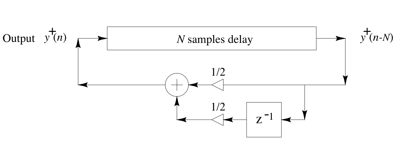
In DWGs, the propagation of the traveling waves is simulated using delay lines. At each sample step, losses occur, but if the loss is a linear operation, it can be commuted out of the individual samples and be applied cumulatively to the output of the delay line.

The model of the loss should be frequency-dependent. With the simplest possible loss filter, we obtain a simulation diagram that looks like this:

This might look familiar as the basic structure of the Karplus-Strong algorithm for plucked string synthesis. In fact, the Karplus-Strong algorithm can be seen as a simple DWG. We’ll look at applying the same methods as before to find the parameters of this model that best fit a given sound using gradient descent.

The transfer function of the basic Karplus-Strong algorithm as shown before is

\[H(z) = \frac{1}{1 - g\cdot(z^{-N} + z^{-N-1})},\]

where \(N\) is the length of the delay line corresponding to the modeled string and controls pitch, and \(g\) is the feedback gain, which controls the decay time of the sound.

We’ll implement this transfer function in the frequency domain for more efficient estimation, and in the time domain for the final result.

import torch
import torchaudio
import IPython.display as ipd
import matplotlib.pyplot as plt

class KarplusStrong(torch.nn.Module):

    def __init__(self, delay_len, n_fft=2048):
        super().__init__()
        self.delay_gain = torch.nn.Parameter(torch.tensor(0.0))
        self.delay_len = delay_len
        
        # for frequency sampling
        self.z = torch.exp(1j * torch.linspace(0, torch.pi, n_fft // 2 + 1))         

        # random excitation
        self.exc = torch.zeros(n_fft)
        self.exc[:delay_len] = torch.rand(delay_len) - 0.5
        self.exc_fft = torch.fft.rfft(self.exc)

    # scale delay gain to [0.9, 1.0]
    def scaled_gain(self):
        return torch.sigmoid(self.delay_gain) * 0.1 + 0.9    
    
    # forward pass: synthesis in the frequency domain
    def forward(self):
        z = self.z
        
        delay_gain = self.scaled_gain()
        
        # sample transfer function
        numer = 1.
        denom = (1 - delay_gain * (0.5 * z ** (-self.delay_len) + 0.5 * z ** (-self.delay_len - 1)))
        
        # filter excitation in frequency domain
        return self.exc_fft * numer / denom

    # also provide method for time domain synthesis
    def time_domain_synth(self, n_samples):

        delay_gain = self.scaled_gain()

        # populate filter coefficients for IIR filter
        a_coeffs = torch.zeros(self.delay_len + 2)        
        a_coeffs[0] = 1
        a_coeffs[self.delay_len] = -delay_gain * 0.5
        a_coeffs[self.delay_len + 1] = -delay_gain * 0.5
    
        b_coeffs = torch.zeros(self.delay_len + 2)
        b_coeffs[0] = 1
    
        # pad or truncate self.exc to n_samples
        if self.exc.shape[0] < n_samples:
            audio = torch.cat([self.exc, torch.zeros(n_samples - self.exc.shape[0])])
        else:
            audio = self.exc[:n_samples]
    
        audio = torchaudio.functional.lfilter(audio, a_coeffs, b_coeffs, clamp=False)
        return audio

# let's have a listen
synth = KarplusStrong(80)
audio = synth.time_domain_synth(32000)
ipd.Audio(audio.detach(), rate=16000)

Let’s now load an acoustic guitar sound file from the NSynth dataset. We’ll try to have our Karplus-Strong model mimic this sound. Since it is a very simple model, we won’t get too close of a match, but we should be able to tune the decay time.

As mentioned before, pitch estimation with gradient descent can be tricky, so we’ll infer the length of the delay line from the pitch of the recording: At MIDI note 51, it’s about 155.56 Hz. With a sample rate of 16000 Hz, this corresponds to a delay of 102.8 samples. We’ll round this to 103 samples. More accuracy could be achieved by using fractional delays, but we’ll keep it simple here.

audio, sample_rate = torchaudio.load("guitar_acoustic_030-051-127.wav") 
audio = audio[0]

sr = 16000

# how many points used in sampling the transfer function
nfft = 4096

# fix random excitation
torch.manual_seed(0)

model = KarplusStrong(delay_len=103, n_fft=nfft)

print("Original:")
ipd.display(ipd.Audio(audio, rate=sr))

print("Synthesized:")
ipd.display(ipd.Audio(model.time_domain_synth(sr * 4).detach(), rate=sr))

Original:

Synthesized:

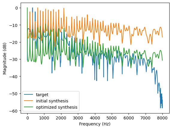
This doesn’t sound close at all. Let’s see if we can once again use gradient descent to find a better value for \(g\) and match the decay time. We’ll use L1 loss on the normalized log magnitudes of the spectrum:

def to_log_mag(freq_response, rel_to_max=True, eps=1e-7):
    mag = torch.abs(freq_response)
    if rel_to_max:
        div = torch.max(mag)
    else:
        div = 1.0
    return 10 * torch.log10(mag / div + eps)


def loss_fn(y, y_hat):
    y_mags = to_log_mag(y)
    y_hat_mags = to_log_mag(y_hat)

    return torch.mean((y_mags - y_hat_mags).abs())

We’re all set for optimization!

# calculate truncated fft
target = torch.fft.rfft(audio, n=nfft)

fftfreqs = torch.fft.rfftfreq(nfft, 1 / sr)

plt.plot(fftfreqs, to_log_mag(target.detach()), label="target")
plt.plot(fftfreqs, to_log_mag(model().detach()), label="initial synthesis")

optim = torch.optim.Adam(model.parameters(), lr=1e-2)
for i in range(1000):
    optim.zero_grad()
    loss = loss_fn(target, model())
    loss.backward()
    optim.step()
    

plt.plot(fftfreqs, to_log_mag(model().detach()), label="optimized synthesis")
plt.legend()
plt.ylabel("Magnitude (dB)")
plt.xlabel("Frequency (Hz)")
plt.show()

print("Audio after optimization:")
td_out = model.time_domain_synth(audio.shape[0]).detach()
ipd.display(ipd.Audio(td_out, rate=sr))

Audio after optimization: